
1-click AWS Deployment 1-click Azure Deployment 1-click Google Deployment
Overview
WEKA is an open source softwarewhich provides tools for data pre processing, implementation of several Machine Learning algorithms, and visualization tools so that we can develop machine learning techniques and apply them to real-world data mining problems. Following diagram will explain what WEKA offers:
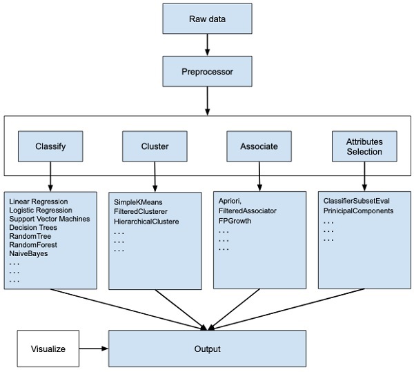
First, you will start with the raw data collected from the field. This data may contain several null values and irrelevant fields. You use the data preprocessing tools provided in WEKA to cleanse the data.Then, you would save the preprocessed data in your local storage for applying ML algorithms.Next, depending on the kind of ML model that you are trying to develop you would select one of the options such as Classify, Cluster, or Associate. The Attributes Selection allows the automatic selection of features to create a reduced dataset.Note that under each category, WEKA provides the implementation of several algorithms. You would select an algorithm of your choice, set the desired parameters and run it on the dataset.WEKA would give you the statistical output of the model processing. It provides you a visualization tool to inspect the data.The various models can be applied on the same dataset. You can then compare the outputs of different models and select the best that meets your purpose.
Weka is a data mining/machine learning application. The purpose of this article is to teach you how to use the Weka Explorer, classify a dataset with Weka, and visualize the results.
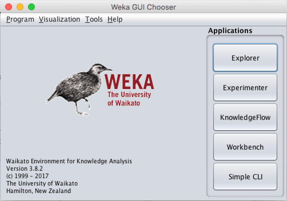
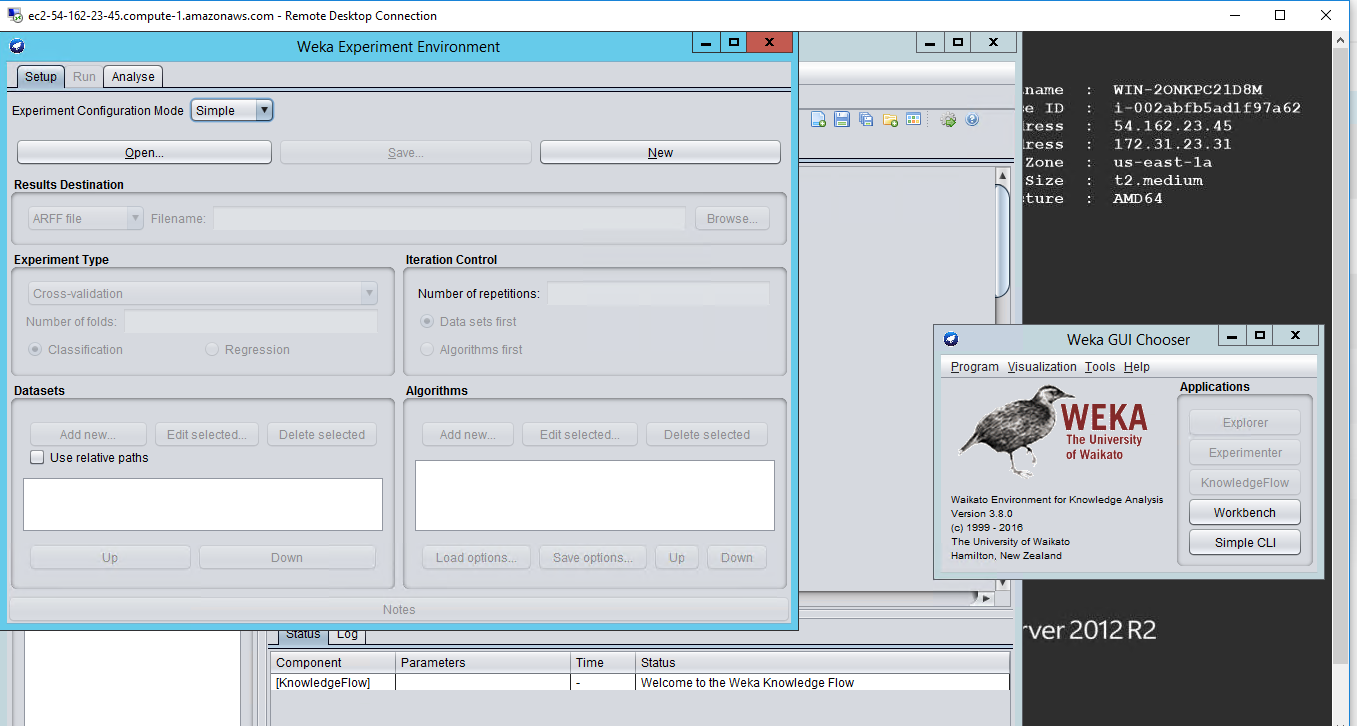
- Simple CLI is a simple command line interface provided to run Weka functions directly.
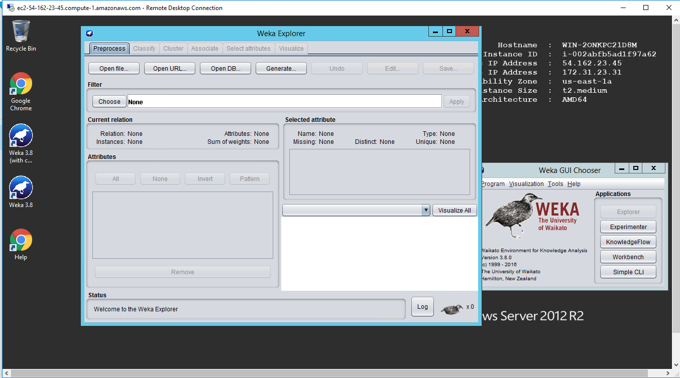
2. Explorer is an environment to discover the data.
3. Experimenter is an environment to make experiments and statistical tests between learning schemes.
4. KnowledgeFlow is a Java-Beans based interface for tuning and machine learning experiments.
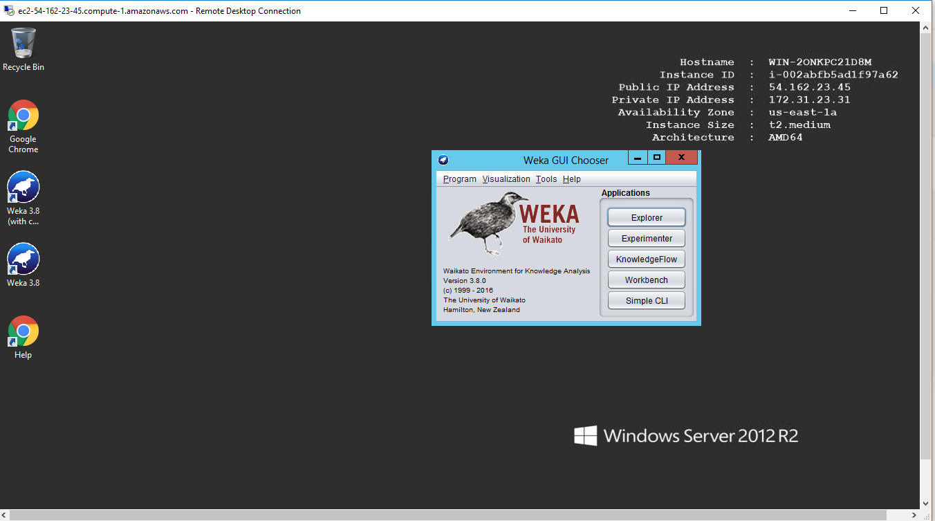
I will use ‘Explorer’ for the exercises. Just click the Explorer button to switch to the Explorer section.
Pre-processing
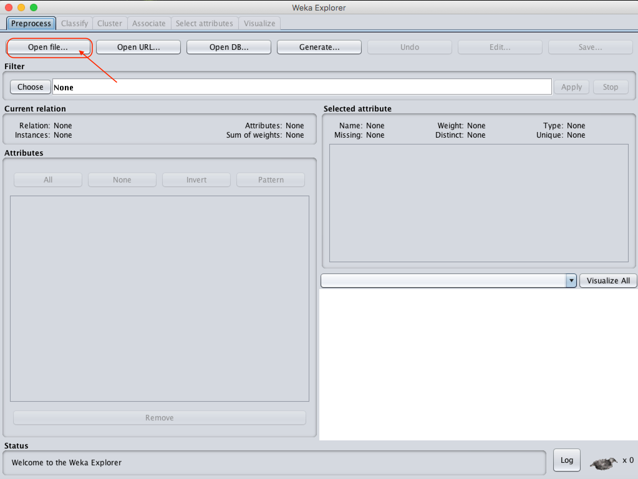
Most of the time, the data wouldn’t be perfect, and we would need to do pre-processing before applying machine learning algorithms on it. Doing pre-processing is easy in Weka. You can simply click the “Open file” button and load your file as certain file types: Arff, CSV, C4.5, binary, LIBSVM, XRFF; you can also load SQL db file via the URL and then you can apply filters to it. However, we won’t need to do pre-processing for this post since we’ll use a dataset that Weka provides for us.
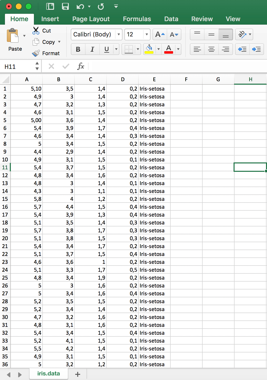
If your data type is in xls format like in Figure 2.1, you have to convert the file. I’ll use the Iris dataset to illustrate the conversion:
- Convert your .xls to .csv format
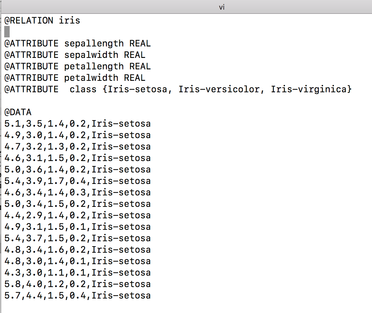
- Open your CSV file in any text editor and first add @RELATION database_name to the first row of the CSV file
- Add attributes by using the following definition: @ATTRIBUTE attr_name attr_type. If attr_type is numeric you should define it as REAL, otherwise you have to add values between curly parentheses. Sample images are below.
- At last, add a @DATA tag just above on your data rows. Then save your file with .arff extension. You can see the illustration in Figure 2.2.
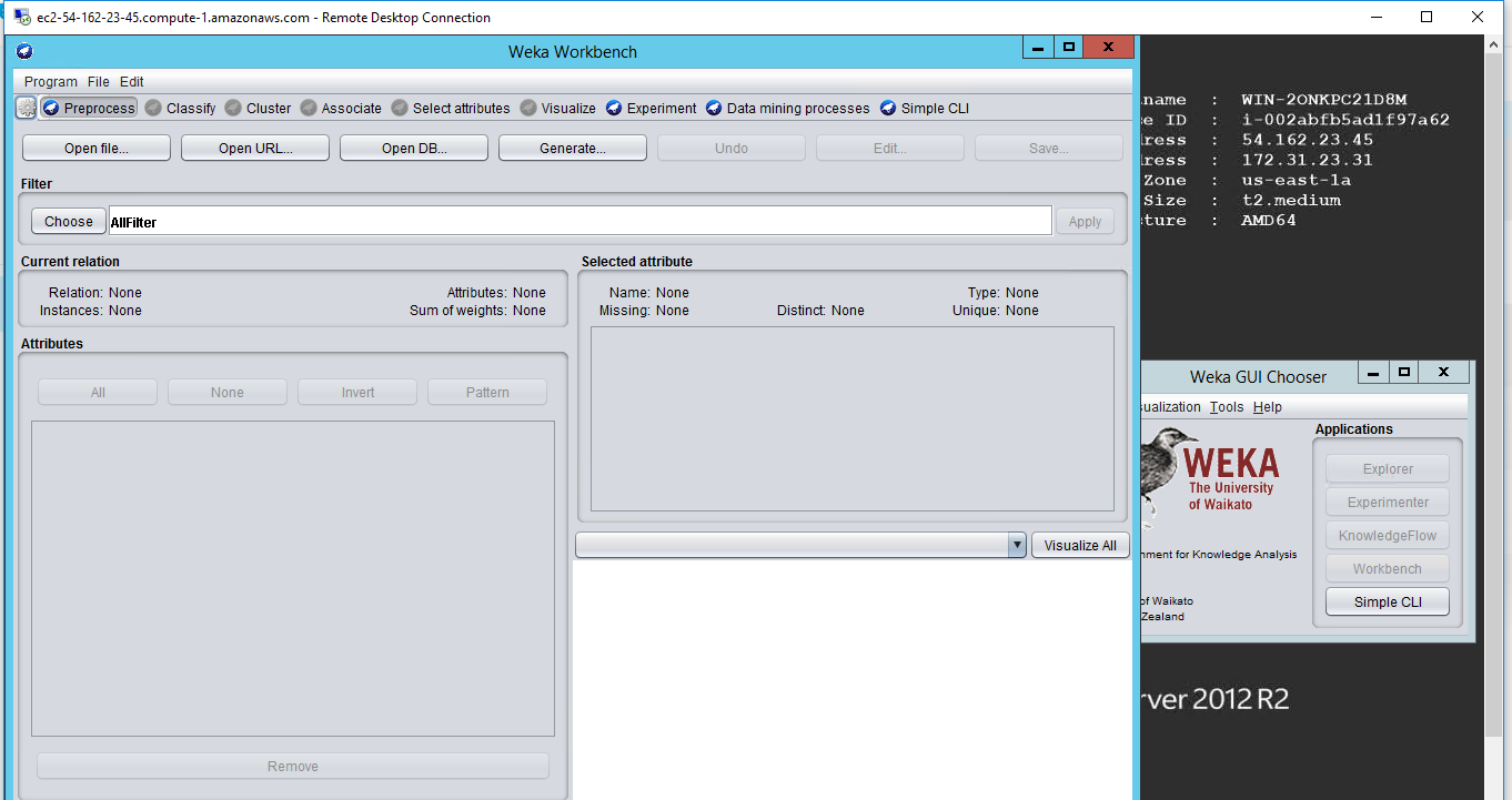
Load Your Data
Click the “Open file” button from the Pre-process section and load your .arff file from your local file system. If you couldn’t convert your .csv to .arff, don’t worry, because Weka will do that instead of you.
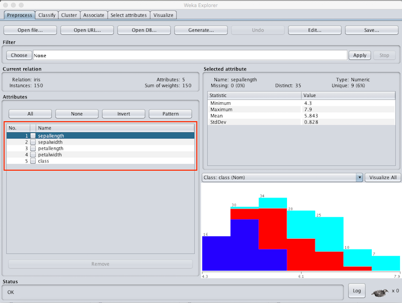
If you could follow all the steps so far, you can load your data set successfully and you’ll see attribute names (it is illustrated at the red area on above images). The pre-process stage is named as Filter in Weka, you can click the ‘Choose’ button from Filter and apply any filter you want. For example, if you would like to use Association Rule Mining as a training model, you have to dissociate numeric and continuous attributes. To be able to do that you can follow the path: Choose -> Filter -> Supervised -> Attribute -> Discritize
Classification
The concept of classification is basically distribute data among the various classes defined on a data set. Classification algorithms learn this form of distribution from a given set of training and then try to classify it correctly when it comes to test data for which the class is not specified. The values that specify these classes on the dataset are given a label name and are used to determine the class of data to be given during the test.
For this tutorial we will use Iris dataset to illustrate the usage of classification with Weka. You can download the dataset from here. Since Iris dataset doesn’t need pre-processing, we can do classification directly by using it. Weka is a good tool for beginners; it includes a tremendous amount of algorithms in it. After you load your dataset, by clicking the Classify section you can switch to another window which we will talk about in this post.
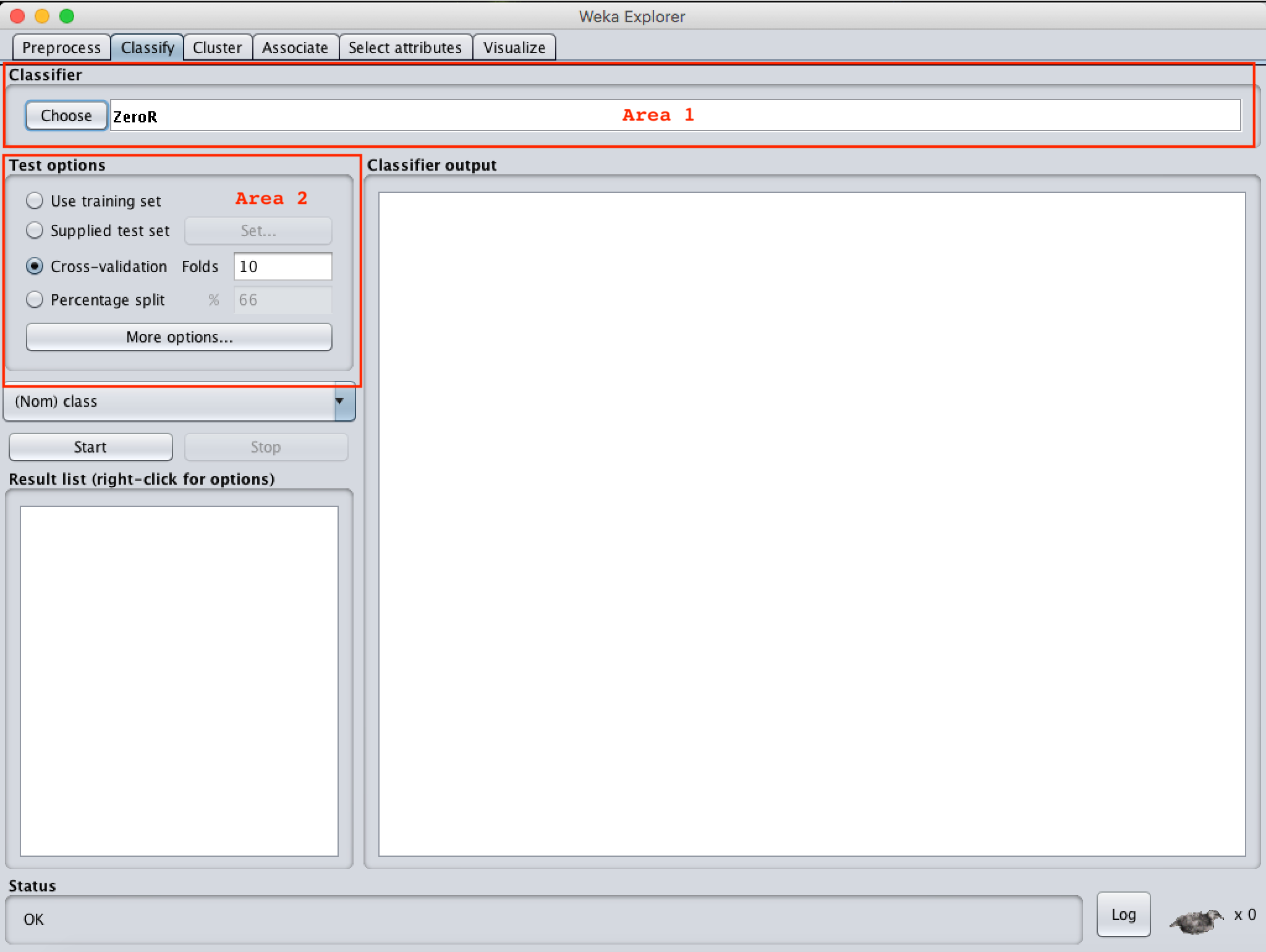
ZeroR is the default classifier for Weka. But since ZeroR algorithm’s performance are not good for Iris dataset, we’ll switch it with the J48 algorithm known for its very good success rate for our dataset. By clicking the Choose button from Area 1 on the above Figure 4.1, a new algorithm can be selected from list. J48 algorithm is inside of trees directory in the Classifier list. Before running the algorithm we have to select the test options from Area 2. Test options consist of 4 options:
- Use training set: Classifies your model based on the dataset which you originally trained your model with.
- Supplied test set: Controls how your model is classified based on the dataset you supply from externally. Select a dataset file by clicking the Set button.
- Cross-validation: The cross validation option is a widely used one, especially if you have limited amount of datasets. The number you enter in the Fold section are used to divide your dataset into Fold numbers (let’s say it is 10). The original dataset is randomly partitioned into 10 subsets. After that, Weka uses set 1 for testing and 9 sets for training for the first training, then uses set 2 for testing and the other 9 sets for training, and repeat that 10 times in total by incrementing the set number each time. In the end, the average success rate is reported to the user.
- Percentage split: Divide your dataset into train and test according to the number you enter. By default the percentage value is 66%, it means 66% of your dataset will be used as training set and the other 33% will be your test set.

By clicking the text area, (the arrow on Figure 4.2) you can edit the parameters of the algorithm according to your needs.
I chose the 10 fold cross validation from Test Options using the J48 algorithm. I chose my class feature from the drop down list as class and click the “Start” button from Area 2 in Figure 4.3. According the result, the success rate is 96%, you can see it from the Classifier Output has shown at Area 1 in Figure 4.3.
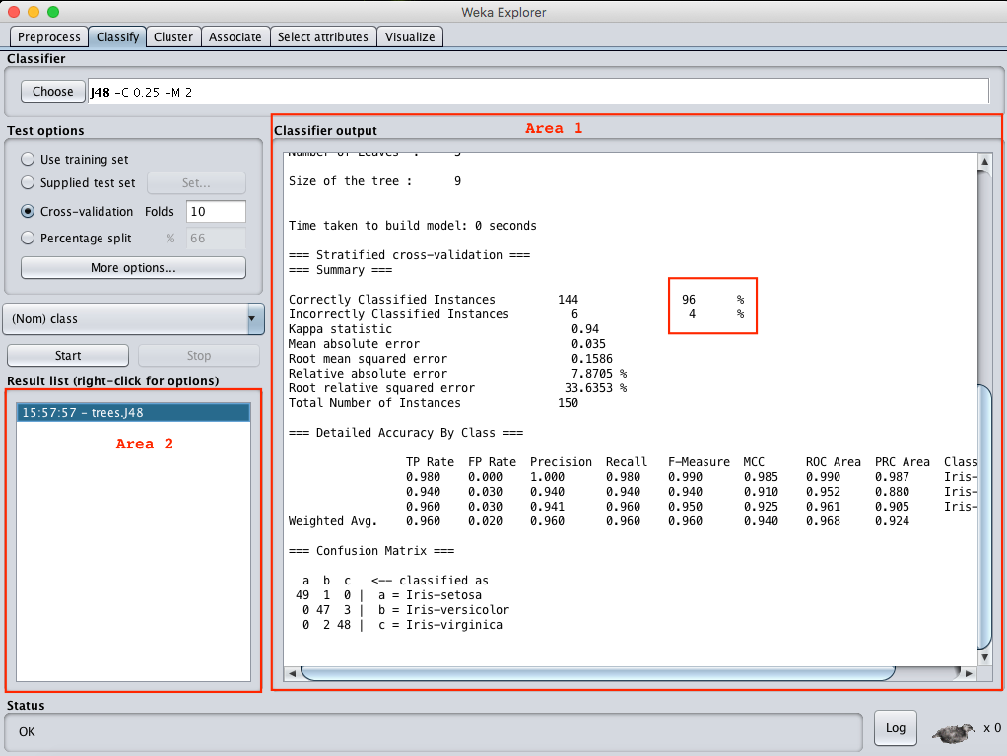
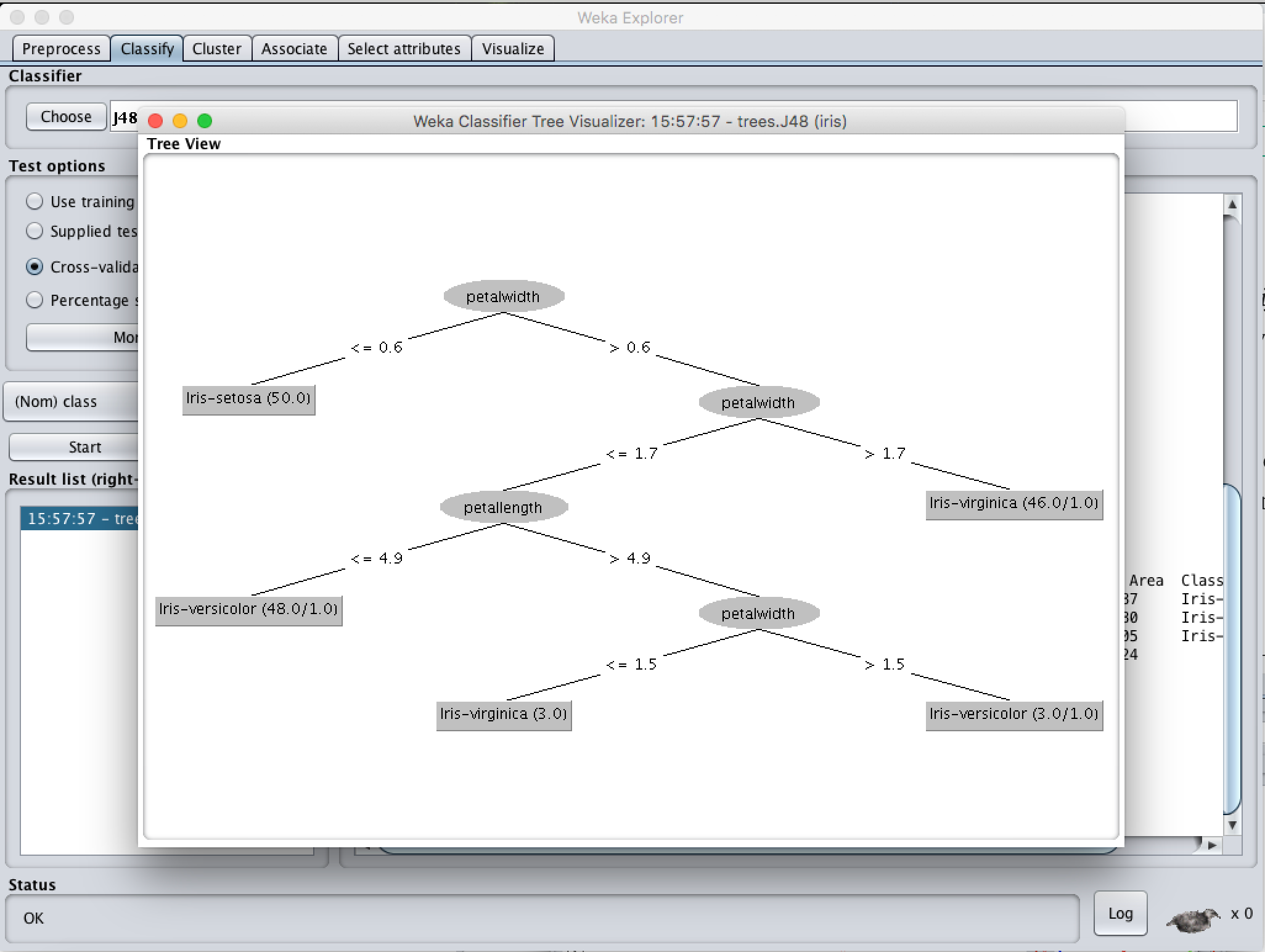
Run Information in Area 1 will give you detailed results as you can see in Figure 4.4. It consists of 5 parts; the first one is Run Information, which gives detailed information about the dataset and the model you used. As you can see in Figure 4.4, we used J48 as a classification model, our dataset was Iris dataset and its features are sepallength, sepalwidth, petallength, petalwidth, class. Our test mode is 10-fold cross-validation. Since J48 is a decision tree, our model created a pruned tree. As you can see on the tree, the first branching happened on petallength which shows the petal length of the flowers, if the value is smaller or equal to 0.6, the species is Iris-setosa, otherwise there is another branch that checks another specification to decide the species. In tree structure, ‘:’ represents the class label.
The Classifier Model part illustrates the model as a tree and gives some information about the tree, like number of leaves, size of the tree, etc. Next is the stratified cross-validation part and it shows the error rates. By checking this part you can see how successful your model is. For example, our model correctly classified 96% of the training data and our mean absolute error rate is 0.035, which is acceptable according to Iris dataset and our model.

You can see a Confusion Matrix and detailed Accuracy Table at the bottom of the report. F-Measure and ROC Area rates are important for the models and they are developed according to a confusion matrix. A confusion matrix represents the True Positive, True Negative, False Positive and False Negative rates, which I explain next. If you already understand Confustion Matrices you can directly skip to the Visualizing the Result part.
Confusion Matrix
True Positive means that the actual class of classification is equal to the class your model set. Lets say you have a dataset which consist of patients’ information, some of them have cancer, some of them don’t. You’re creating a model to diagnose patients automatically in terms of their blood analysis results. So you give a patient’s information to your model and your model’s result shows the patient has cancer. In this case, our positive result is being healthy and negative result is finding cancer. Then you check the actual experts’ results with yours, and if he/she isn’t diagnosed with cancer, you had a False Negative (FN). If the expert said that the patient does not have cancer at all, it means that your model result is wrong. A False Positive (FP) means you found a positive result but it is actually negative, like if your model found that the patient is healthy, but the expert said that he/she has cancer. A False Negative (TN) happens when the result is negative but in reality it is positive. If your model and the expert say that he/she is healthy, then your result counts as True Positive (TP). It might seem a bit confusing at first sight, but while you’re using it you’ll find these results easily. Confusion matrices consist of these 4 values.
Visualizing the Result
If you’d like to visualize this results you can use graphic presentations as you can see in below Figure 4.5.
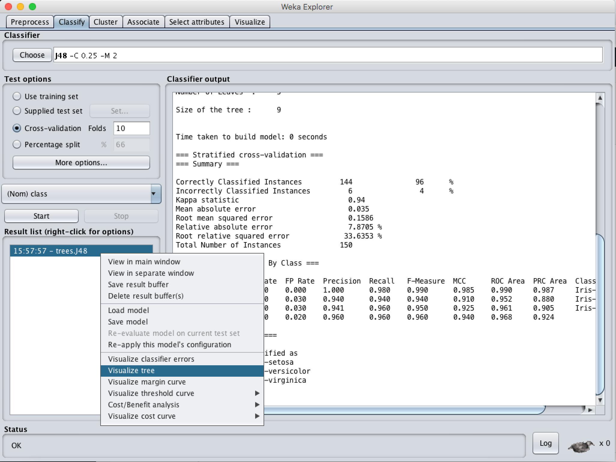
By right clicking Visualize tree you’ll see your model’s illustration like in Figure 4.6.
If you’d like to see classification errors illustrated, select Visualize Classifier Errors in same menu. By sliding jitter (you can see in Area 1 at Figure 4.6) you can see all samples on coordinate plane. The X plane represents predicted classifier results, the Y plane represents actual classifier results. Squares represent wrongly classified samples. Stars represent true classified samples. Blue colored ones are Iris-setosa, red colored stars are Iris-versicolor, green ones Iris-virginica species. So, red square means our model classified this sample as Iris versicolor but it supposed to be Iris virginica.
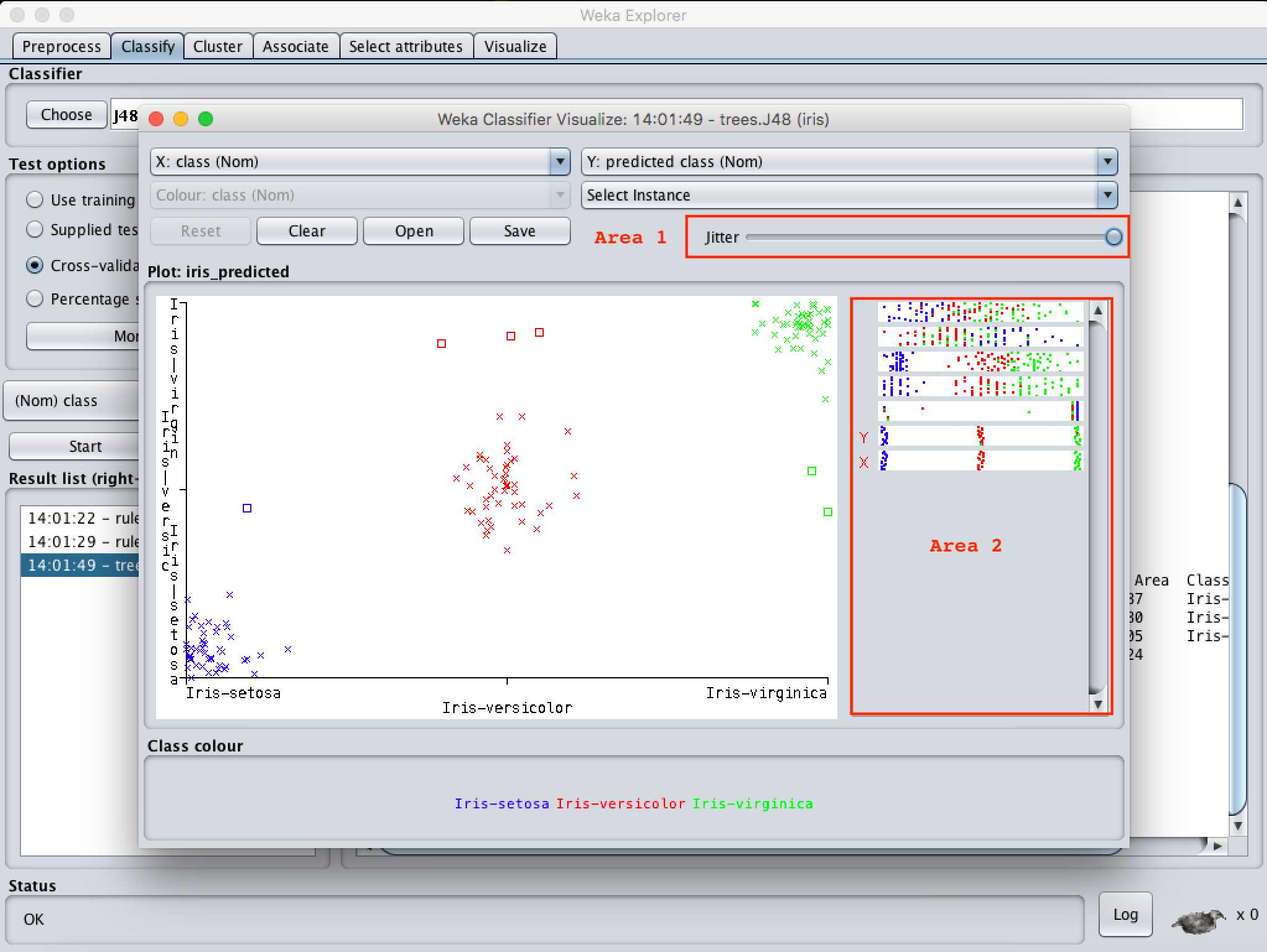
If you click on one of the squares, you can see more detailed information. I clicked one of the blue ones as shown in Figure 4.8, and saw which sample is classified wrong in detail. But, why would we want to see wrongly classified samples in detail?

We have various samples which have to classified in machine learning. Sometimes, looking by yourself at the samples, it gives you basic ideas to make your classifier model more robust or find outliers which are irrelevant information for the data you use, etc. So, however we call it as machine learning, most of the time it depends a human to control the data in datasets.
- Regression
- Clustering
- Association
- Data pre-processing
- Classification
- Visualisation
The features of Weka are shown below


Weka contains tools for data pre-processing, classification, regression, clustering, association rules, and visualization. It is also well-suited for developing new machine learning schemes.
Weka is owned by Weka (https://sourceforge.net/projects/weka/) and they own all related trademarks and IP rights for this software.
Weka is open source software issued under the GNU General Public License.
Weka on cloud for AWS
Features
Five features of Weka are:
- Open Source: It is released as open source software under the GNU GPL. It is dual licensed and Pentaho Corporation owns the exclusive license to use the platform for business intelligence in their own product.
- Graphical Interface: It has a Graphical User Interface (GUI). This allows you to complete your machine learning projects without programming.
- Command Line Interface: All features of the software can used from the command line. This can be very useful for scripting large jobs.
- Java API: It is written in Java and provides a API that is well documented and promotes integration into your own applications. Note that the GNU GPL means that in turn your software would also have to be released as GPL.
- Documentation: There books, manuals, wikis and MOOC courses that can train you how to use the platform effectively
Major Features of Weka
-
- Machine Learning
-
- Data Mining
-
- Preprocessing
-
- Classification
-
- Regression
-
- Clustering
-
- Association rules
-
- Attribute selection
-
- Experiments
-
- Workflow
- Visualization
AWS
Installation Instructions For Windows
Note: How to find PublicDNS in AWS
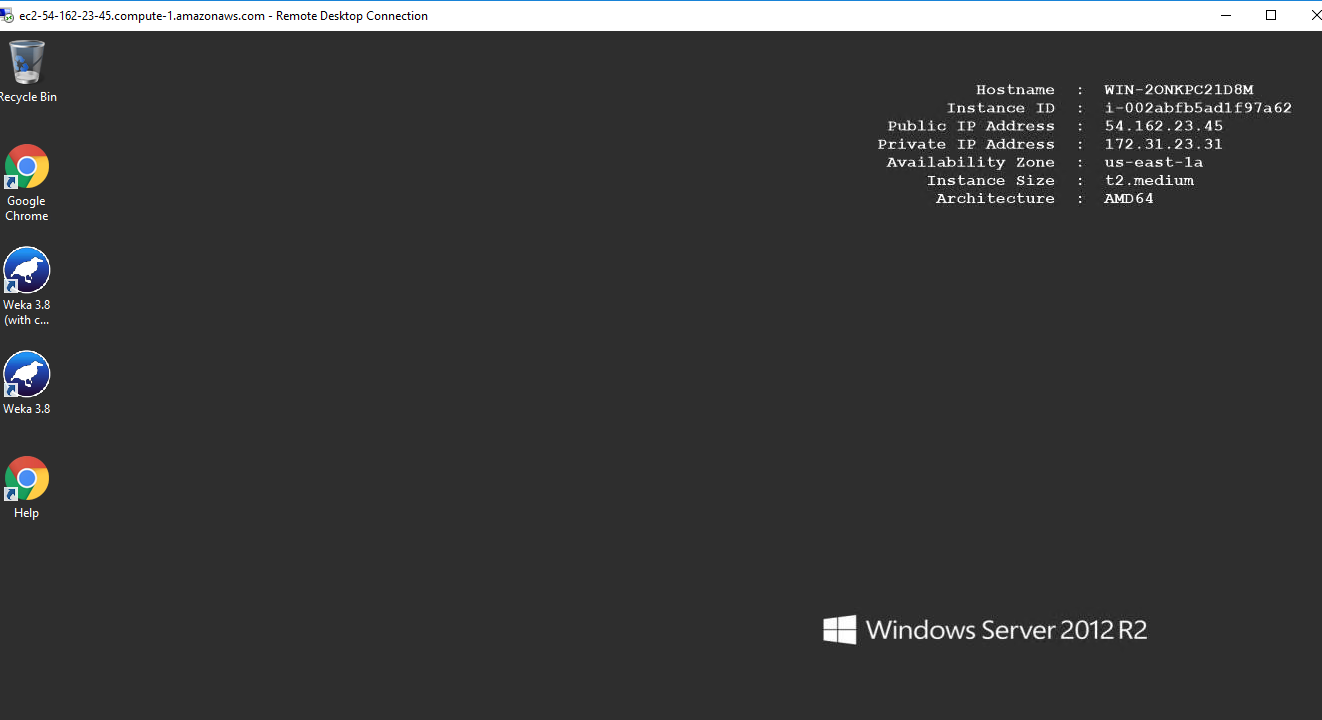
Step 1) RDP Connection: To connect to the deployed instance, Please follow Instructions to Connect to Windows instance on AWS Cloud
1) Connect to the virtual machine using following RDP credentials:
- Hostname: PublicDNS / IP of machine
- Port : 3389
Username: To connect to the operating system, use RDP and the username is Administrator.
Password: Please Click here to know how to get password .
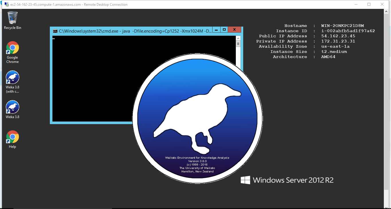
Step 2) Click the Windows “Start” button and select “All Programs” and then point to Weka.
Step 3) Other Information:
1.Default installation path: will bein your root folder “C:\Program Files\Weka-3-8”
2.Default ports:
- Windows Machines: RDP Port – 3389
- Http: 80
- Https: 443
Note: Click on Desktop icon – Press start then App will open in the browser.
Configure custom inbound and outbound rules using this link
Installation Step by Step Screenshots
Installation Instructions For Windows
Installation Instructions for Windows
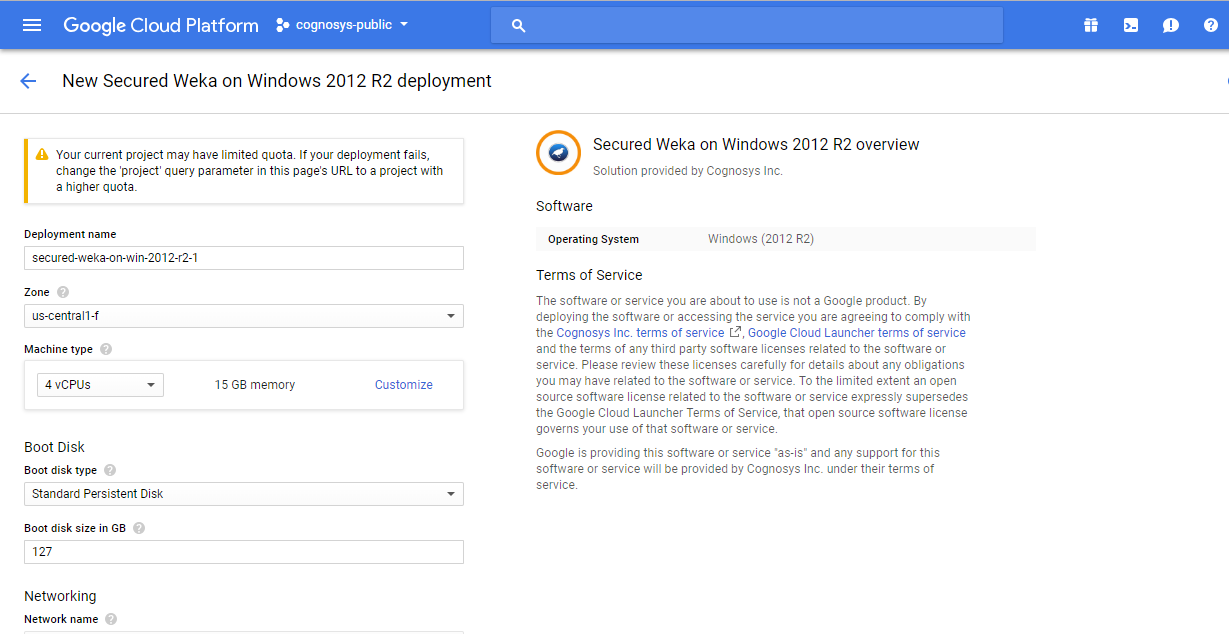
Step 1) VM Creation:
- Click the Launch on Compute Engine button to choose the hardware and network settings.
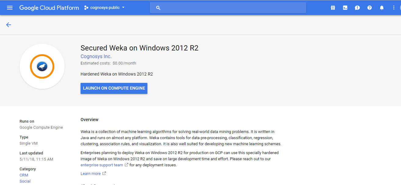

- You can see at this page, an overview of Cognosys Image as well as estimated cost of running the instance.
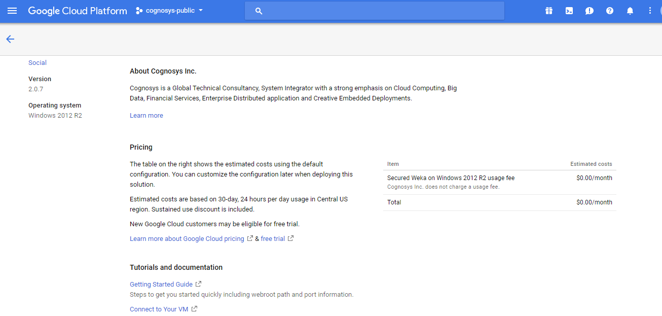

- In the settings page, you can choose the number of CPUs and amount of RAM, the disk size and type etc.

Step 2) RDP Connection: To initialize the DB Server connect to the deployed instance, Please follow Instructions to Connect to Windows instance on Google Cloud
Step 2) Click the Windows “Start” button and select “All Programs” and then point to Weka.
Step 3) Other Information:
1.Default installation path: will bein your root folder “C:\Program Files\Weka-3-8”
2.Default ports:
- Windows Machines: RDP Port – 3389
- Http: 80
- Https: 443
Note: Click on Desktop icon – Press start then App will open in the browser.